Value at Risk: Matricies
We define a number of methods for producing matrices in VolatilityAbstract.java.
getCorrelationMatrix(double[][] matrix)getCovarianceMatrix(double[][] matrix)getCholeskyDecompositionMatrix(double[][] matrix)
All of these methods returns an \(N \times N\) matrix for a portfolio of \(N\) stocks.
Percentage Changes
Suppose our portfolio contains multiple stocks, say GOOG, MSFT, and AAPL.
We will need to compute a vector of historical percentage changes for each of these. We can combine each of these vectors to produce a matrix of price changes.
In Analytical.java, HistoricalSimulation.java, and MonteCarlo.java we instantiate this matrix as a two dimensional array:
double[][] matrix = double[countAsset][size];
where countAsset is the number of stock symbols in our portfolio and size is the number of percentage changes in our data.
Variance Covariance Matrix
The value of each element is simply the variance between two vectors of percentage changes.
\[\begin{bmatrix} \sigma^2_{GOOG,GOOG} & \sigma^2_{GOOG,MSFT} & \sigma^2_{GOOG,AAPL}\\ \sigma^2_{MSFT,GOOG} & \sigma^2_{MSFT,MSFT} & \sigma^2_{MSFT,AAPL}\\ \sigma^2_{AAPL,GOOG} & \sigma^2_{AAPL,MSF} & \sigma^2_{AAPL,AAPL} \end{bmatrix}\]In our implementation, we simply step through each element of our matrix and invoke getVariance().
public double[][] getCovarianceMatrix(double[][] matrix) {
    int numCol = matrix.length;
    double[][] covarianceMatrix = new double[numCol][numCol];

    for (int i = 0; i < numCol; i++) {
        for (int j = 0; j < numCol; j++)
            covarianceMatrix[i][j] = getVariance(matrix[i], matrix[j]);
    }
    return covarianceMatrix;
}
The covariance matrix for a portfolio of GOOG, MSFT, and AAPL stocks looks something like:
\[\begin{bmatrix} 2.694056173665337E-4 & 2.1361059045418314E-4 & 1.709980427330677E-4\\ 2.1361059045418314E-4 & 2.669503258565737E-4 & 1.7039293114741037E-4\\ 1.709980427330677E-4 & 1.7039293114741037E-4 & 2.6718851085657364E-4 \end{bmatrix}\]Note that getVariance() is an abstract class and could be instantiated in a number of ways.
The above output was computed from an equal weighted variance estimate.
Correlation Matrix
In the below figure we illustrate the correlation of two stocks, \(X\) and \(Y\). Moving from left to right, we see examples of:
- full positive correlation
- independence
- full negative correlation
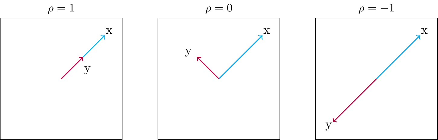
Each length is the volatility of the historical percentage change of each stock.
The correlation coefficient is calculated as:
\[\rho = \frac{cov(\Delta\Pi_1,\Delta\Pi_2)}{std(\Delta\Pi_1)\cdot std(\Delta\Pi_2)}\]In our implementation of getCorrelationMatrix(), we iterate through each matrix element and assign correlation by invoking both getVariance() and getVolatility() at each step.
public double[][] getCorrelationMatrix(double[][] matrix) {
    int numCol = matrix.length;
    double[][] correlationMatrix = new double[numCol][numCol];

    for (int i = 0; i < numCol; i++) {
        for (int j = 0; j < numCol; j++) {
            double covXY = getVariance(matrix[i], matrix[j]);
            double sigmaX = getVolatility(matrix[i], matrix[i]);
            double sigmaY = getVolatility(matrix[j], matrix[j]);
            correlationMatrix[i][j] = covXY / (sigmaX * (sigmaY));
        }
    }
    return correlationMatrix;
}
The correlation matrix for a portfolio of GOOG, MSFT, and AAPL stocks looks something like:
\[\begin{bmatrix} 1.0 & 0.7965338367423306 & 0.6373513737349931\\ 0.7965338367423306 & 1.0 & 0.6380099568758332\\ 0.6373513737349931 & 0.6380099568758332 & 1.0 \end{bmatrix}\]The unit diagonal makes sense - any random variable is fully correlated with itself.
Cholesky Decomposition
In all our scalar volatility estimates, we have been computing volatility as the square root of variance.
But what if we need to return a multivariate (i.e. a matrix) estimate of volatility?
We do in fact need this when simulating multiple stock price changes in MonteCarlo.java.
We need a way of finding the square root of a matrix \(\Sigma\). But there is no direct way of doing this.
Our approach is to take the Cholesky decomposition to approximate \(\Sigma\). This gives us a lower triangular matrix \(L\) in which all elements above the diagonal are zero. The product of \(L\) with its transpose is \(\Sigma\).
\[\Sigma = LL'\]Consider the following matrix \(A\), which is symmetric and positive definite as an example:
\[A = \begin{bmatrix} a_{11} & a_{12} & a_{13}\\ a_{21} & a_{22} & a_{23}\\ a_{31} & a_{32} & a_{33} \end{bmatrix}\]We need to find \(L\) such that \(A=LL^T\). Writing this out looks like:
\[\begin{bmatrix} a_{11} & a_{12} & a_{13}\\ a_{21} & a_{22} & a_{23}\\ a_{31} & a_{32} & a_{33} \end{bmatrix} = \begin{bmatrix} l_{11} & 0 & 0\\ l_{21} & l_{22} & 0\\ l_{31} & l_{32} & l_{33} \end{bmatrix} \begin{bmatrix} l_{11} & l_{21} & l_{31}\\ 0 & l_{22} & l_{32}\\ 0 & 0 & l_{33} \end{bmatrix} = \begin{bmatrix} l_{11}^2 & l_{21}l_{11} & l_{31}l_{11}\\ l_{21}l_{11} & l_{21}^2 + l_{22}^2 & l_{31}l_{21}+l_{32}l_{22}\\ l_{31}l_{11} & l_{31}l_{21}+l_{32}l_{22} & l_{31}^2+l_{32}^2+l_{33}^2 \end{bmatrix}\]Then we obtain the following formulas for \(L\):
above the diagonal
\[L_{ii} = \Bigg( a_{ii}-\sum_{k=1}^{i-1}L_{ik}^2\Bigg)^{1/2}\]below the diagonal
\[L_{ji}=\frac{1}{L_{ii}}\Bigg(a_{ij}-\sum_{k=1}^{i-1}L_{ik}L_{jk}\Bigg)\]Our implementation is as follows:
public double[][] getCholeskyDecomposition(double[][] matrix) {
    double[][] covarianceMatrix = getCovarianceMatrix(matrix);
    int numCol = matrix.length;
    double[][] choleskyMatrix = new double[numCol][numCol];

    for (int i = 0; i < covarianceMatrix.length; i++)
        for (int j = 0; j <= i; j++) {
            Double sum = 0.0;
            for (int k = 0; k < j; k++)
                sum += choleskyMatrix[i][k] * choleskyMatrix[j][k];
            if (i == j)
                choleskyMatrix[i][j] = Math.sqrt(covarianceMatrix[i][j] - sum);
            else
                choleskyMatrix[i][j] = (covarianceMatrix[i][j] - sum) / choleskyMatrix[j][j];
        }
    return choleskyMatrix;
}
The Cholesky decomposition for a portfolio of GOOG, MSFT, and AAPL stocks looks something like:
\[\begin{bmatrix} 0.016443923964552982 & 0.0 & 0.0\\ 0.013040234356363926 & 0.009897342218550691 & 0.0\\ 0.010440391951585325 & 0.0035291225401465846 & 0.012116136426183954 \end{bmatrix}\]