With Monte Carlo we can simulate a distribution by way of randomly generating a whole bunch of numbers. In Central Limit Theorem, the distribution of the sum of a large number of small contributions is approximately Gaussian.
Stock prices can be described as a random walk. That is, a stock price is the linear combination of a number of infinitessimally small changes otherwise known as the Wiener Process. Each change is randomly sampled from the standard Gaussian distribution \(\phi(0,1)\). Our predicted stock price is where ever we end up at the end of the random walk.
With Monte Carlo, we simply predict a large number of stock prices and calculate the pay-off for prediction. Then we average these pay-offs and apply discounting to obtain our predicted option price.
Formula
We use the Generalised Wiener process to generate a random walk. This recursive formula describes this process:
\[x(t + \Delta t) = x(t) + \mu\Delta t + \sigma dz\]Where:
- \(dz\) is the basic Wiener Process.
- \(\Delta t\) is a time step of some very small duration
- \(x_t\) is the stock price at the current time step
- \(x_{t + \Delta t}\) is the stock price at the next time step
Note: \(x(0)\) is our initial stock price.
Basic Wiener Process
The Wiener Process is a particular type of Markov Process with mean change 0 and variance rate of 1 per year.
We sample randomly from the standard Gaussian distribution and multiply by \(\sqrt{T}\).
\[\Delta z = \epsilon \sqrt{\Delta t}\]where \(\epsilon_i\) is our random sample.
Values of \(\Delta z\) at different time slices, \(\Delta t\), are independent.
Random Walk
Consider the below illustration. We a see a simple random walk with approximately \(N=6\) intervals of \(\Delta t\).
As you can see, at each step we move up or down.
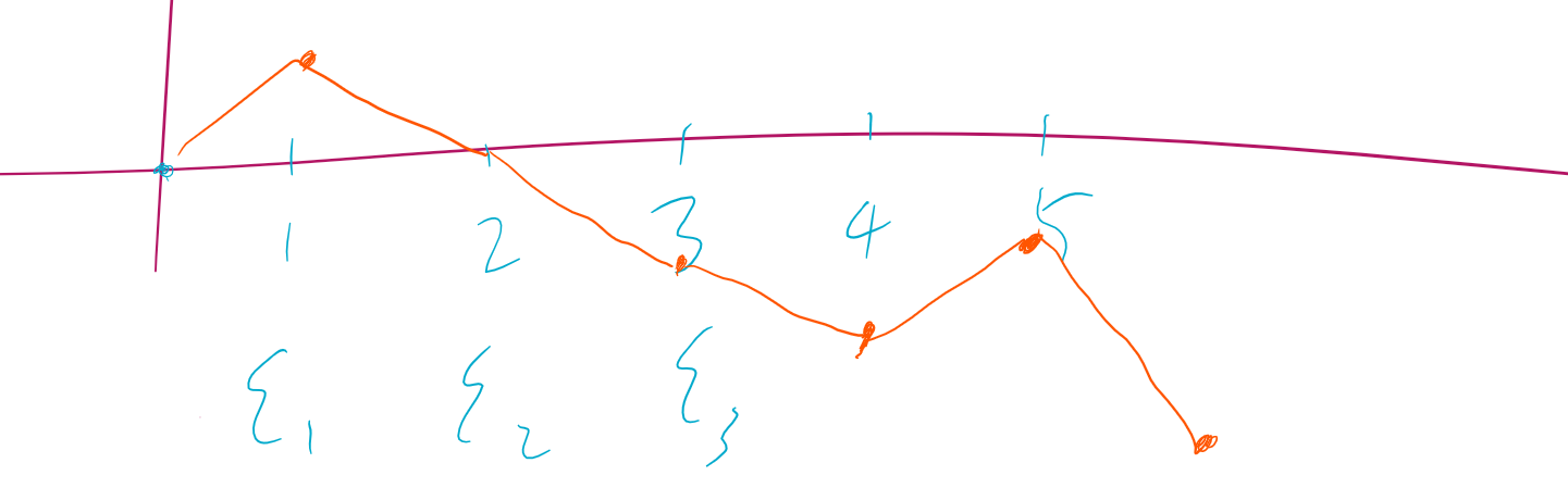
At the end of the walk (\(t=T\)), we can describe the position of random variable \(z\) as:
\[z(T) - z(0) = \sum_{i=1}^N \epsilon_i \sqrt{\Delta t}\]Our final position is calculated as the linear combination of every step in the walk.
Epsilon
We define epsilon as a random variable \(\epsilon_i\) sampled from the standard gaussian (mean 0, standard devition 1).
\(\epsilon_i \sim \phi(0,1)\).
This means that the value of epsilon is going to be somewhere between -1 and +1. On average, this value is going to be \(\approx 0\).
The sign of our value dictates the up/down direction of our step.
Scaling
Our Random Walk has the duration \(T - 0\). But we would like our steps \(\Delta t\) to be as small as possible. The result is a really fine random walk.
\[\Delta t = \frac{T}{N}\]We therefore want \(N\) to be as large as possible.
Suppose we want to simulate the change in a stock price over the next year, \(T=1\). It would make sense to divide this time horizon by \(N=365\) such that each timeslice \(\Delta t\) represents one day.
Java
Sampling in Java
How do we generate epsilon in Java?
We use the java.util.Random class. When instantiated, this class will generate an iterable collection of pseudorandom numbers. This collection is governed by a seed, which is set by the constructor Random().
According to the Java doc, this seed is unlikely to collide with any previous seed.
Random random = new Random();
We want to sample from the Gaussian distribution so we use the method nextGaussian() to return the next pseudorandom sample from the Gaussian distribution.
double epsilon = random.nextGaussian();
Basic Weiner Process
Translating all this to a method is rather simple:
    public double basicWeinerProcess(double dt) {
        Random epsilon = new Random();
        // sample from random Gaussian of mean 0 and sd 1
        double dz = epsilon.nextGaussian()*Math.sqrt(dt);
        // return a step. value dz, size dt.
        return dz;
    }
Random Walk
MonteCarlo is an abstract class, which means it can contain abstract methods.
simulateRandomWalk is an abstract method that returns two different results.
This is because we are interested in computing both Asian and European payoffs.
… for European payoff
A European payoff is defined as follows for calls and puts respectively:
\[f_{call} = max(S_T - X, 0)\\ f_{put} = max(X - S_T, 0)\]As such, at the end of our random walk, we need only return the stock price at maturity, \(t=T\).
public double simulateRandomWalk
	(int N, double S0, double dt, double interest, double sigma) {
	double St = S0;
    for (int t = 1; t < N; t++) {
		double dz = basicWeinerProcess(dt);
        St = St + (interest * St * dt) + (sigma * St * dz);
    }
    return St;
}
…for Asian payoff
In computing the payoff for Asian options, we use the average stock price over the entire time horizon instead of the stock price at maturity.
\[f_{call} = max(S_{avg} - X, 0)\\ f_{put} = max(X - S_{avg}, 0)\]The implementation is similar to the above case except we keep a partial total of stock prices in the while loop.
At the end of the loop, we take this total and divided by the number of steps. In doing so, we return the average stock price.
public double simulateRandomWalk
	(int N, double S0, double dt, double interest, double sigma) {
	double St = S0;
    double partialTotal = S0;
    for (int t = 1; t < N; t++) {
    	double dz = basicWeinerProcess(dt);
        St = St + (interest * St * dt) + (sigma * St * dz);
        partialTotal += St;
    }
    return partialTotal/N;
}